%matplotlib inline

Landmark-based multi-sample single-cell data analysis

# Table of contents * Read Data * Generate Sample Embeddings * Samaple-based Analysis

Get started

• To run this notebook, you have to download the preterm_unstim.h5ad data from this link, and put it into the data folder under the project root.

• Install our sclkme package and other dependencies using the pip command:

  • pip install sclkme phate statannotations

If there are any questions or problems, please push an issue under the git repo at https://github.com/CompCy-lab/scLKME.

# Uncomment and run this cell if you're on Colab or Kaggle
# !pip install sclkme phate statannotations

# load the packages needed
%reload_ext autoreload

# load the dependencies
import sclkme   # load the sclkme package
import scanpy as sc
import anndata as ad
import os.path as osp
import pandas as pd

import matplotlib.pyplot as plt
import matplotlib.ticker as ticker
import matplotlib as mpl
mpl.rcParams["figure.facecolor"] = 'white'
import seaborn as sns

from pathlib import Path
from matplotlib.pyplot import rc_context

sc.settings.verbosity = 1
sc.settings.set_figure_params(dpi=80, facecolor='white')
sc.logging.print_header()

scanpy==1.9.3 anndata==0.9.2 umap==0.5.4 numpy==1.23.5 scipy==1.10.1 pandas==1.5.3 scikit-learn==1.3.2 statsmodels==0.14.0 python-igraph==0.10.8 pynndescent==0.5.10

Read the data

data_root = osp.join(osp.dirname(osp.abspath("__file__")), "../../data")
adata_path = osp.join(Path(data_root).resolve(), "preterm_unstim.h5ad")

# read the .h5ad data
adata = sc.read_h5ad(adata_path)

# show the available fields in the data
print(adata)

AnnData object with n_obs × n_vars = 400000 × 38
    obs: 'Sample_ID', 'Plate_ID', 'Stim', 'FCS_File', 'Class', 'Category', 'Gestational.Age', 'X_64_sketch', 'X_128_sketch', 'X_256_sketch', 'X_512_sketch'
    uns: 'X_128_sketch', 'X_256_sketch', 'X_512_sketch', 'X_64_sketch', 'kme', 'neighbors', 'sampleXmeta', 'umap'
    obsm: 'X_kme', 'X_umap'
    obsp: 'connectivities', 'distances'

Generate sample-based embeddings

The landmark matrix X_anchor is an n_landmark by d matrix, where the rows are landmark cells and the columns are the embedding features, which can be raw gene/protein features or extracted features, like PCA.

# cell sketching with n_landmark=512 landmarks
sclkme.tl.sketch(adata, n_sketch=512, use_rep="X", key_added="X_512", method="kernel_herding")

adata_sketch = adata[adata.obs['X_512_sketch']]
# get the precomputed anchor cells
X_anchor = adata_sketch.X.copy()

print(X_anchor)

[[0.06662848 4.0252423  3.2229903  ... 1.0307382  0.3225428  0.1303769 ]
 [1.4203637  4.2610917  2.4013813  ... 0.         0.         0.        ]
 [0.6415793  4.6462755  3.3441646  ... 0.5812172  1.8201672  0.        ]
 ...
 [0.40527838 4.117027   3.5839536  ... 0.65212226 0.49960423 0.        ]
 [0.         4.126464   4.0653095  ... 0.         0.         0.        ]
 [0.8006469  4.363835   3.8853781  ... 1.1542339  3.6173465  1.370174  ]]

Run the kernel mean embedding using the api provided by the sclkme package.

This api is pretty much similar to standard interface in the scanpy ecosystem. For the parameters,

• partition_key: the column name of sample ids in the adata.obs dataframe.

• X_anchor: the landmakr matrix

• use_rep: the indicated representation to be used. Note: the representation should have identical dimensions as the landmark matrix.

By default, the output sample embeddings are stored in adata.uns['kme']['{partition_key}_kme'].

# run kernel mean embedding 
sclkme.tl.kernel_mean_embedding(adata, partition_key="Sample_ID", X_anchor=X_anchor, use_rep='X')

# show sample embeddings
# pd.set_option('display.max_columns', 6)

adata.uns['kme']['Sample_ID_kme'].head()

	X_kme_0	X_kme_1	X_kme_2	X_kme_3	X_kme_4	X_kme_5	X_kme_6	X_kme_7	X_kme_8	X_kme_9	...	X_kme_502	X_kme_503	X_kme_504	X_kme_505	X_kme_506	X_kme_507	X_kme_508	X_kme_509	X_kme_510	X_kme_511
Sample_ID
CB10T	0.568137	0.516859	0.647542	0.362659	0.454447	0.589324	0.600191	0.483299	0.593141	0.372919	...	0.442153	0.381815	0.524996	0.485006	0.636462	0.608896	0.575762	0.410888	0.420804	0.497886
CB11-AP	0.509170	0.522249	0.514000	0.407897	0.471045	0.468700	0.494871	0.397684	0.471713	0.352793	...	0.489170	0.431116	0.510078	0.458123	0.627160	0.547009	0.525865	0.480013	0.464187	0.459410
CB11-BP	0.510515	0.504690	0.529104	0.450097	0.510501	0.471506	0.499843	0.442229	0.475539	0.339085	...	0.485501	0.461806	0.523375	0.478437	0.643484	0.571422	0.552002	0.465727	0.453075	0.474139
CB12P	0.452424	0.521209	0.406091	0.513055	0.545144	0.346239	0.387355	0.392161	0.352428	0.385342	...	0.520035	0.469245	0.400201	0.337749	0.529777	0.432825	0.409252	0.503371	0.491035	0.336433
CB14P	0.507396	0.620306	0.459013	0.399986	0.441434	0.413071	0.416108	0.335017	0.411108	0.540626	...	0.599916	0.393721	0.405664	0.324018	0.508857	0.435034	0.397705	0.593167	0.599104	0.334227

5 rows × 512 columns

Sample-based data analysis

# acquire sample-level meta data
sample_obs = adata.obs[["Sample_ID", "Class", "Category", "Gestational.Age"]].groupby(by="Sample_ID", sort=False).agg(lambda x: x[0])

adata_sample = ad.AnnData(adata.uns['kme']['Sample_ID_kme'], obs=sample_obs)

/Users/haidyi/Documents/proj/scLKME/.venv/lib/python3.10/site-packages/anndata/_core/anndata.py:121: ImplicitModificationWarning: Transforming to str index.
  warnings.warn("Transforming to str index.", ImplicitModificationWarning)

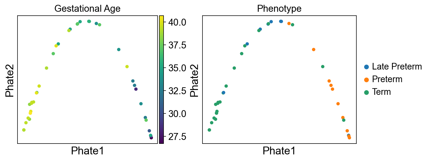
Visualize sample embeddings using PHATE

sc.external.tl.phate(adata_sample, n_pca=10, k=9, t="auto",
                     random_state=0, mds_solver="smacof", verbose=True, copy=False)

fig, axes = plt.subplots(1, 2, figsize=(9, 3.5))

sc.external.pl.phate(adata_sample, color=['Gestational.Age'], title="Gestational Age", color_map="viridis", size=100, ax=axes[0], show=False)
sc.external.pl.phate(adata_sample, color=['Category'], title="Phenotype", size=100, ax=axes[1], show=False)

for ax in axes:
    ax.set_xlabel("Phate1", fontsize=16)
    ax.set_ylabel("Phate2", fontsize=16)

plt.show()

/Users/haidyi/Documents/proj/scLKME/.venv/lib/python3.10/site-packages/pygsp/filters/simpletight.py:79: SyntaxWarning: "is" with a literal. Did you mean "=="?
  if kerneltype is 'sf':
/Users/haidyi/Documents/proj/scLKME/.venv/lib/python3.10/site-packages/pygsp/filters/simpletight.py:82: SyntaxWarning: "is" with a literal. Did you mean "=="?
  elif kerneltype is 'wavelet':

Calculating PHATE...
  Running PHATE on 40 observations and 512 variables.
  Calculating graph and diffusion operator...
    Calculating PCA...
    Calculated PCA in 0.01 seconds.
    Calculating KNN search...
    Calculating affinities...
  Calculated graph and diffusion operator in 0.03 seconds.
  Calculating optimal t...
    Automatically selected t = 23
  Calculated optimal t in 0.02 seconds.
  Calculating diffusion potential...
  Calculating metric MDS...
  Calculated metric MDS in 0.01 seconds.
Calculated PHATE in 0.08 seconds.

/Users/haidyi/Documents/proj/scLKME/.venv/lib/python3.10/site-packages/phate/phate.py:186: FutureWarning: k is deprecated. Please use knn in future.
  warnings.warn("k is deprecated. Please use knn in future.", FutureWarning)
/Users/haidyi/Documents/proj/scLKME/.venv/lib/python3.10/site-packages/phate/phate.py:190: FutureWarning: a is deprecated. Please use decay in future.
  warnings.warn("a is deprecated. Please use decay in future.", FutureWarning)
/Users/haidyi/Documents/proj/scLKME/.venv/lib/python3.10/site-packages/sklearn/manifold/_mds.py:298: FutureWarning: The default value of `normalized_stress` will change to `'auto'` in version 1.4. To suppress this warning, manually set the value of `normalized_stress`.
  warnings.warn(
/Users/haidyi/Documents/proj/scLKME/.venv/lib/python3.10/site-packages/scanpy/plotting/_tools/scatterplots.py:392: UserWarning: No data for colormapping provided via 'c'. Parameters 'cmap' will be ignored
  cax = scatter(

Visualize sample embeddings using diffusion map

sc.pp.neighbors(adata_sample, n_neighbors=8, use_rep="X", key_added="diffmap_nn")
sc.tl.diffmap(adata_sample, n_comps=3, neighbors_key="diffmap_nn")

sc.pl.diffmap(adata_sample, color=["Gestational.Age", "Category"], size=100,
              palette=sc.pl.palettes.vega_20_scanpy, color_map="viridis", components=['2,3'])

/Users/haidyi/Documents/proj/scLKME/.venv/lib/python3.10/site-packages/scanpy/plotting/_tools/scatterplots.py:392: UserWarning: No data for colormapping provided via 'c'. Parameters 'cmap' will be ignored
  cax = scatter(

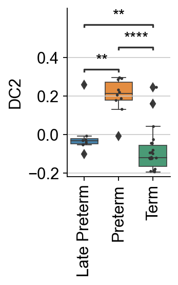
T-test on the coordinates of diffusion map

from statannotations.Annotator import Annotator

diffmap_df = sc.get.obs_df(adata_sample, keys=['Category', 'Gestational.Age'], obsm_keys=[('X_diffmap', 1)])

g = sns.catplot(x="Category", y="X_diffmap-1", data=diffmap_df, kind="box",
                legend=False, linewidth=0.8, boxprops=dict(alpha=.9), height=3, aspect=0.8, sharey=False)

axes = g.axes.flatten()
for ax, y in zip(g.axes.flatten(), ["X_diffmap-1"]):
    sns.stripplot(x="Category", y=y, data=diffmap_df, color=".2", size=2.5, jitter=True, ax=ax)
    annot = Annotator(ax, [("Term", "Late Preterm"), ("Late Preterm", "Preterm"), ("Term", "Preterm")],
                      data=diffmap_df, x="Category", y=y, order=["Late Preterm", "Preterm", "Term"])
    annot.configure(test='Mann-Whitney', text_format='star', loc='inside', verbose=2)
    annot.apply_test()
    _, test_results = annot.annotate()
    

for ax in axes:
    ax.set_title(None)
    ax.set_xticklabels(labels=ax.get_xticklabels(), rotation=90)

axes[0].set_ylabel("DC2")
axes[0].set_yticks([-0.2, 0.0, 0.2, 0.4])

g.set_xlabels("")

plt.show()

p-value annotation legend:
      ns: 5.00e-02 < p <= 1.00e+00
       *: 1.00e-02 < p <= 5.00e-02
      **: 1.00e-03 < p <= 1.00e-02
     ***: 1.00e-04 < p <= 1.00e-03
    ****: p <= 1.00e-04

Late Preterm vs. Preterm: Mann-Whitney-Wilcoxon test two-sided, P_val:2.057e-03 U_stat=7.000e+00
Preterm vs. Term: Mann-Whitney-Wilcoxon test two-sided, P_val:5.227e-05 U_stat=2.100e+02
Late Preterm vs. Term: Mann-Whitney-Wilcoxon test two-sided, P_val:9.928e-03 U_stat=1.420e+02